
Data filtering can be an immensely helpful function to use when it comes to sifting through large amounts of data. However, when it comes to accurately executing the function, there are 5 excel filter tips to keep in mind so as not to miscalculate:
- Ascending/Descending Order
One of the most common Excel filter tips beginners are offered would be to data sort in ascending or descending order. That can be accomplished by locating the ‘Data tab’ and choosing ‘Sort & Filter group’ or using keyboard shortcuts (CTRL + SHIFT + L). Users can then select where to apply the filter to, whereby they can choose to sort by ascending order (Sort Smallest to Largest) or descending order (Largest to Smallest).
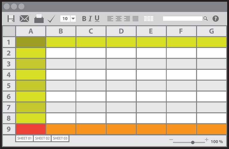
- Colour
Filtering data by colour is an option Microsoft Excel has available as well. Do note that this option will only be available after the user has applied cell colours, font colours or conditional formatting. Once users have selected the ‘Sort & Filter’ function, drop down arrows will be visible. Select the drop down arrow located on the table headers and select ‘Filter by colour’. This will then make available the options in which you can filter by.
- More than two criteria
Users are also able to filter excel lists while using more than two criterias. This would rely on the use of the ‘Advanced filter’. This can similarly be located under the ‘Data tab’. Choose ‘Filter’ and ‘Advanced Filter’ when the option becomes available. Once this is accomplished, users will then be able to select the list range option and insert their desired list range. Users can also select the ‘Criteria Range’ option and insert their desired criteria range before authorising the change by choosing ‘OK’.
- Select Cells
Data filtering can also be done by specific cells, according to factors like- value, colour and font colour. Select ‘Filter’ and choose ‘Filter by selected cell’s value’, after that simply choose the cell for filter application and authorise the application. This should successfully apply the filter to the selected cell.
- Saving Filter Criteria
For this to work successfully, it is advisable to make use of ‘Custom View’ for future quick selection purposes as it allows users to save display/print settings in a custom view icon. Select the ‘File tab’ and locate ‘Options’. The ‘Excel Options’ window should appear upon that. After which, select ‘Choose Commands From’ and choose ‘Customise ribbon’. Locate ‘View’, ‘Custom views’ and simply select ‘Add’ to create a shortcut. Now that this has been created, save the filtering criteria by selecting a cell containing the desired criteria and locate the ‘Filter option’. Making use of the drop down lists present, select ‘Custom views’ and add it in.
These are 5 basic Excel data filter tips to remember while using the functions. With consistent practice, you will be able to perform this with relative ease and get the data results you need without having to resort to tedious measures.